🇬🇧 English · 🇪🇸 Español

Sovereign-risk policy brief: reentry, volatility and persistence

This is an illustrative brief on PureMacro's public calibration of the short-term Arellano (2008) model, not a claim about any country. Nothing is fitted to targets: the baseline is the calibration whose solver and grid convergence are checked in the Arellano replication guide, and each scenario moves one parameter away from it.

Question

How do three features of a borrowing economy change its sovereign risk? The features are the probability of regaining market access after a default (θ), the volatility of income (σ_y) and the persistence of income (ρ_y). The outcomes are average debt (the debt chosen in repayment quarters as a percentage of mean quarterly income; divide by four for an approximate debt-to-annual-GDP ratio), the mean spread, the frequency of default, the volatility of spreads, and the value of market access: the permanent consumption gain, in percent, that would make an economy in financial autarky with no default cost as well off as one that can borrow starting from zero debt, with both values averaged over the long-run income distribution.

Answer

In this illustrative model, starting from the public calibration and moving one parameter at a time from its low to its high value: a higher reentry probability (θ 0.15 → 0.5) lowers average debt from 6.808% of mean quarterly income to 2.374% of mean quarterly income; raises the mean spread from 1.860% to 5.127%; raises default frequency from 1.807% a year to 4.879% a year; and lowers the value of market access from 0.094% of consumption to 0.023% of consumption. A higher income volatility (σ_y 0.02 → 0.03) lowers average debt from 4.048% of mean quarterly income to 3.529% of mean quarterly income; raises the mean spread from 3.053% to 3.110%; raises default frequency from 2.933% a year to 2.989% a year; and lowers the value of market access from 0.053% of consumption to 0.035% of consumption. A higher income persistence (ρ_y 0.9 → 0.97) raises average debt from 2.521% of mean quarterly income to 5.996% of mean quarterly income; raises the mean spread from 2.398% to 3.434%; raises default frequency from 2.323% a year to 3.311% a year; and raises the value of market access from 0.036% of consumption to 0.066% of consumption. Each number is a mean over 16 simulated paths of 500,000 quarters; the table gives its 95% interval and its grid change.

The levels for θ = 0.5 and ρ_y = 0.97 (marked † in the table) are not grid-converged by the registered criterion; the directions of their effects are, since the grid changes are far smaller than the differences between scenarios.

The volatility effect is not monotone. At σ_y = 0.02 / 0.025 / 0.03 the mean spread is 3.053 / 3.114 / 3.110 % and default frequency 2.933 / 2.989 / 2.989 % a year: all of the rise comes between 0.02 and 0.025, and from 0.025 to 0.03 neither rises (paired baseline → σ_y = 0.03 change -0.0033 ± 0.0012 pp for the spread and -0.001 ± 0.011 pp for default, with 95% intervals). These effects are also of the order of the grid changes in the table, so this calibration says little about their sign.

Results

The table reports, for each scenario on the 6,401 x 641 grid validated for the baseline, the mean across 16 simulated paths of 500,000 quarters (after a 1,000-quarter burn), ± the half-width of its 95% Student-t interval across paths. The number in parentheses, Δ, is the paired change from the 3,201 x 641 grid to the 6,401 x 641 grid, path by path with the same seeds. The registered tolerance for that change is 0.10 for each of the four moments (the replication study's grid tolerance, in the same units). No tolerance is registered for the value of market access, so its Δ is reported without a pass or fail. A † marks a scenario where at least one moment's change, plus its 95% half-width, does not fit inside the tolerance; such rows are reported, not dropped.

Scenario	Debt (% of mean quarterly income)	Mean spread (%)	Default (% per year)	Spread SD (pp)	Value of market access (%)
Baseline	3.821 ± 0.025 (Δ +0.006)	3.114 ± 0.005 (Δ -0.022)	2.989 ± 0.029 (Δ -0.027)	2.549 ± 0.005 (Δ -0.034)	0.043 (Δ +0.000)
θ = 0.15	6.808 ± 0.037 (Δ +0.006)	1.860 ± 0.003 (Δ -0.001)	1.807 ± 0.020 (Δ +0.005)	1.829 ± 0.003 (Δ -0.001)	0.094 (Δ +0.000)
θ = 0.5 †	2.374 ± 0.013 (Δ +0.009)	5.127 ± 0.007 (Δ +0.174)	4.879 ± 0.035 (Δ +0.167)	4.429 ± 0.005 (Δ -0.180)	0.023 (Δ +0.000)
σ_y = 0.02	4.048 ± 0.024 (Δ +0.003)	3.053 ± 0.005 (Δ +0.004)	2.933 ± 0.022 (Δ -0.002)	2.508 ± 0.004 (Δ -0.016)	0.053 (Δ +0.000)
σ_y = 0.03	3.529 ± 0.022 (Δ +0.001)	3.110 ± 0.006 (Δ -0.027)	2.989 ± 0.028 (Δ -0.031)	2.529 ± 0.005 (Δ -0.050)	0.035 (Δ +0.000)
ρ_y = 0.9	2.521 ± 0.008 (Δ +0.001)	2.398 ± 0.003 (Δ +0.003)	2.323 ± 0.030 (Δ -0.004)	1.733 ± 0.003 (Δ -0.004)	0.036 (Δ +0.000)
ρ_y = 0.97 †	5.996 ± 0.060 (Δ -0.001)	3.434 ± 0.009 (Δ +0.049)	3.311 ± 0.025 (Δ +0.064)	3.248 ± 0.007 (Δ -0.129)	0.066 (Δ +0.000)

† At least one moment's paired 3,201 x 641 → 6,401 x 641 grid change does not fit the registered 0.10 tolerance (its status is in the record). The row is reported, not dropped.

Grid-change status of the rows marked †: θ = 0.5 (Mean spread (%): grid shift exceeds tolerance; Default (% per year): grid shift exceeds tolerance; Spread SD (pp): grid shift exceeds tolerance); ρ_y = 0.97 (Spread SD (pp): grid shift exceeds tolerance).

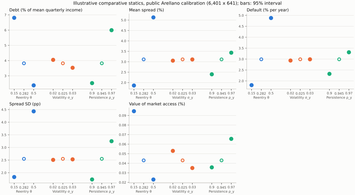
Hollow markers are the shared baseline; whiskers are 95% intervals across paths, most of them narrower than the markers (the value of market access is a solved quantity, without sampling error).

Initial crossed refinement of the sensitive scenarios

The follow-up holds the calibration, 16 seeds, 500,000 periods, burn-in and 0.10 tolerances fixed. It solves all four combinations of 6,401/12,801 debt nodes and 641/1,281 income states. Each cell below is the absolute paired mean change plus its 95% half-width; every moment must be at most 0.10.

Scenario and refinement	Debt	Mean spread	Default	Spread SD	Verdict
θ = 0.5, debt at 1,281 income states	0.003457	0.106816	0.118959	0.174051	Failed
θ = 0.5, income at 12,801 debt nodes	0.016915	0.039766	0.053709	0.054342	Passed
ρ_y = 0.97, debt at 1,281 income states	0.016982	0.030946	0.031479	0.101902	Failed
ρ_y = 0.97, income at 12,801 debt nodes	0.051721	0.032086	0.049175	0.046211	Passed

All eight solves converged, with zero exhaustive-search certification gap and Bellman residual below 9e-12. This isolates the remaining issue to debt-grid moment convergence, rather than an unfinished Bellman solve. For θ = 0.5 the spread-volatility shift itself is −0.167865 pp; more simulation alone cannot remove it. For ρ_y = 0.97 the shift is −0.096678 pp, but its uncertainty bound narrowly misses the criterion. Neither case passes this crossed ladder.

The complete record, including every seed and failed comparison, is tests/fixtures/sovereign_brief/sensitive_grid_initial.json. A further 12,801 → 25,601 debt refinement at both income resolutions is being evaluated under the same tolerances. Its outcome is not implied by these initial results.

python -m tools.reference_validation.check_sovereign_sensitive_grids --output grids_initial
python -m tools.reference_validation.check_sovereign_sensitive_grids --extend-from grids_initial/sensitive_grid_convergence.json --output grids_extended

Both commands must use the same environment. To reuse the bundled initial record instead, its Python, dependency and package versions must match your environment; the extension also checks the numerical source hashes. Historical cases retain their original hashes when the verified income-batching change is used.

Nonuniform refinement for high reentry

A separate study of θ = 0.5 keeps the original debt support [−0.15, 0.33] and the same calibration, seeds, simulation length and tolerances. Of the debt intervals, 5/16 cover saving linearly and 11/16 cover positive borrowing quadratically, concentrating nodes near zero debt. An exploratory coarse pilot motivated this choice; the four large cases, 6,401/12,801 debt nodes crossed with 641/1,281 income states, were specified before their computation. This is our grid design, not a fit to economic targets. The sensitivity to grid placement is consistent with the numerical concern described by Hatchondo, Martinez and Sapriza (2010).

Both required final refinements pass every unchanged 0.10 moment tolerance:

Refinement for θ = 0.5	Debt	Mean spread	Default	Spread SD	Verdict
Debt: 6,401 → 12,801, with 1,281 income states	0.002617	0.003020	0.013577	0.003414	Passed
Income: 641 → 1,281, with 12,801 debt nodes	0.020892	0.052384	0.057949	0.067375	Passed

Cells again report the absolute paired mean change plus its 95% half-width. Every solve converged with zero exhaustive-search certification gap; the largest exhaustive Bellman residual is below 1e-14. The final nonuniform grid gives:

Scenario and grid	Debt (% of mean quarterly income)	Mean spread (%)	Default (% per year)	Spread SD (pp)	Value of market access (%)
θ = 0.5, nonuniform 12,801 × 1,281	2.3550 ± 0.0135	5.1604 ± 0.0073	4.9224 ± 0.0238	3.8115 ± 0.0058	0.0229

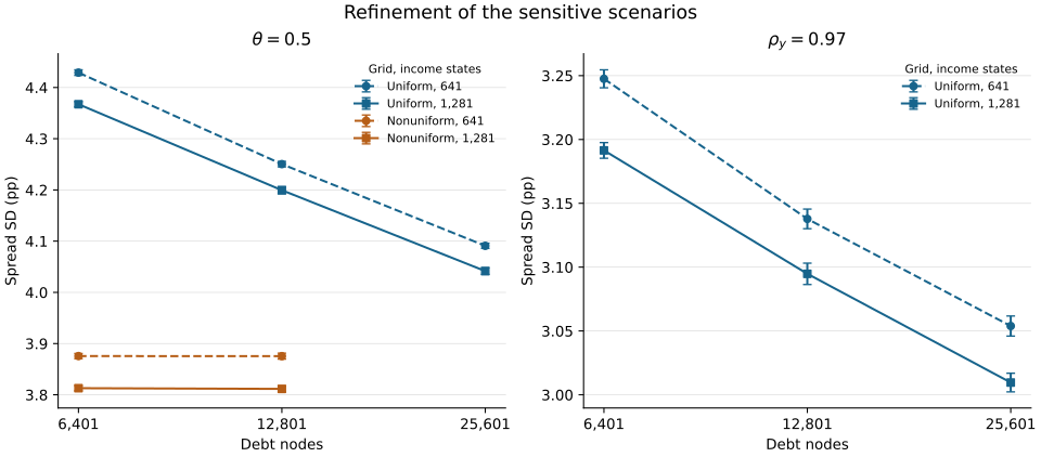
These intervals describe simulation uncertainty. The pass controls changes between the final tested grids in this family, not distance to the infinitely fine limit. The uniform-grid records, including failures, remain alongside this study in tests/fixtures/sovereign_brief/; all nonuniform coordinates, source hashes and per-seed moments are in curved_grid_convergence.json.

python -m tools.reference_validation.check_sovereign_curved_grids --output grids_curved

The public solver accepts the same coordinates through solve_sovereign_default(debt_grid=...).

Run it yourself

This example is included in PureMacro 6.1.0. Install it with pip install puremacro (or from a source checkout) and run a scenario. On the maintainer's workstation the θ = 0.15 solve took about 14 minutes, plus seconds for the measurement, measured under load on a shared machine (load averages 5/13/27); the whole frozen sweep, seven scenarios on both grids, took 6,851 s (1.9 h), with a peak memory of about 3.4 GB:

python -m pip install .
python -m puremacro.examples.first_brief_sovereign --scenario theta=0.15 --output brief_theta015

Scenarios are baseline or theta=…, sigma_y=…, rho_y=…. The output directory receives table.md, table.csv, figure.png, record.json and a manifest.json with the version, grid, seeds and solver certification. For a quick orientation, all seven scenarios on a coarse grid take minutes:

python -m puremacro.examples.first_brief_sovereign --sweep --coarse

The coarse run prints a caveat: its numbers are for orientation only. The main example reproduces the original uniform-grid sweep; use the follow-up commands above for finer grids in the sensitive scenarios. Add --lang es for Spanish output.

Assumptions and limits

• Short-term debt only. One-period bonds, no maturity choice and no restructuring: default wipes out the debt and the economy waits for a random reentry with zero debt.
• Endowment economy. Income is an exogenous log-AR(1) process (Tauchen discretization), so policy cannot change output.
• Arellano penalty. In default, income is min(y, 0.969 ȳ).
• Raw ergodic measurement. The moments come from puremacro.sovereign.ergodic_moments: long simulated paths with the timing of SovereignDefaultResult.simulate, over all repayment quarters, with the solver's linear spread 4 * max(0, yield - r*). Default frequency counts default entries only (not continuing exclusion), as a quarterly hazard among quarters with market access, times 4. The replication guide instead measures 74-quarter windows before defaults with the study's spread convention, and its default frequency is the full-sample 1 - (1 - entries / repayment quarters)^4: compounded, with only repayment quarters in the denominator, where this brief uses the linear 4 * entries / (repayment quarters + entries). The two differences roughly cancel for default (2.989 % here against 2.997 % in the guide at the baseline), but the guide's other numbers differ from these.
• What the grid criterion does not bound. The Δ column bounds the change between two grids, not the distance to the infinitely fine limit; the replication record shows spread SD still drifting monotonically as the grid is refined.
• No empirical claim. These are comparative statics of one calibrated model, not estimates for any country and not policy recommendations.