🇬🇧 English · 🇪🇸 Español

Your first policy brief: tariffs and household welfare

This page walks through one complete policy experiment on public data: the United States levies a 10% tariff on all modeled sectors from China, including services. The brief solves a general-equilibrium trade model on the OECD Inter-Country Input-Output table that ships with puremacro, reports the US welfare change with its price / factor-income / fiscal split, shows how three household groups would be treated, changes one assumption, and states what the numbers do not say. Nothing needs to be downloaded besides the package.

1. Install

You need Python 3.11 or later. This example is included in PureMacro 6.1.0:

python -m pip install puremacro

2. Run

One command runs the brief and writes its tables, figure and record:

python -m puremacro.examples.first_brief_tariffs --output first_brief

The same run from Python:

from puremacro.examples.first_brief_tariffs import run_brief

study = run_brief("first_brief")
print(study["record"]["national"]["ev_pct_consumption"])

The default command writes national.{md,csv,tex}, households.{md,csv,tex}, first_brief.png, headline.json (the numbers below) and manifest.json (package and library versions, the table's citation and SHA-256, solver settings, convergence, timings), plus experiment.{md,csv,tex} when --experiment sigma=<value> is set. Passing --enigh, --trade-elasticity (> 0), or --household-elasticity (> 0) switches to the TradeBriefConfig sensitivity-grid workflow: it computes the headline scenario (defaulting to trade_elasticity=4.0, household_elasticity=1.0, and ENIGH quintiles when --groups is omitted), sweeps sensitivity_trade_elasticities=(2.0, 4.0, 6.0) by sensitivity_household_elasticities=(0.5, 1.0, 1.5), and additionally writes paths.csv, headline.{md,csv,tex}, and headline_es.md (or headline_en.md with --lang es); --experiment is not executed in this mode. Options: --importer, --exporter, --sector (all or one ISIC section A to T), --tariff (0.10 = 10%), --experiment, --groups, --enigh, --trade-elasticity, --household-elasticity, --output, and --lang en|es. The default run takes a few seconds; the solver uses the exact engine with method="equilibrated_newton" and tol=1e-5.

3. Preview: the national result

Equivalent variation (EV) of US consumption, split into the change in purchaser prices, in factor income (wages and capital income) and in fiscal transfers (mostly the tariff revenue, rebated lump sum). The table below is the frozen output of the default run.

Component	million USD	% of baseline consumption
Purchaser prices	-4,646	-0.0277
Factor income	-21,703	-0.1294
Fiscal transfers	32,777	0.1954
Equivalent variation	6,427	0.0383

Positive values are gains. The three lines are an endpoint attribution valued in the model's numeraire; read purchaser prices and factor income together. No retaliation: CHN does not respond.

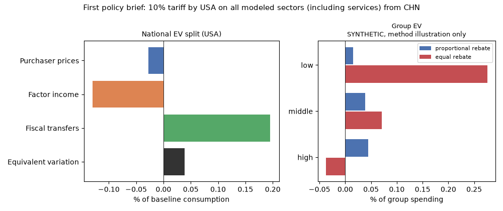
First brief: national EV split and synthetic household groups

Read it this way: higher purchaser prices and lower US factor income together cost 0.157% of baseline consumption. The tariff revenue, rebated lump sum to US residents, adds 0.195%, so the net EV is small and positive (+0.038%). This is not a terms-of-trade gain. With fixed sourcing, Chinese producers do not cut their prices: US wages fall by about 0.14% relative to Chinese wages, and the US terms of trade (export over import unit values, before duties) worsen by about 0.04%. The consumption improvement of 6,427 million USD accompanies changes of -7,096 in investment and -467 in residents' purchases abroad, valued at baseline prices. EV values consumption only: allocation across final uses changes. An independent solver reproduces the result and checks the world resource balance; see the validation. The EV split is an endpoint attribution, not separate causal channels. The result is also unilateral: China does not retaliate here, and a response would change it.

4. One experiment: let firms switch suppliers

python -m puremacro.examples.first_brief_tariffs --experiment sigma=2 --output first_brief_sigma2

sigma is the elasticity of substitution across all country-sector intermediate inputs. The headline uses sigma=0 (Leontief); sigma=2 lets buyers in every country change both source countries and input sectors. It is not an elasticity restricted to origins within the same sector. Final-use baskets stay fixed. The table compares the two:

Measure	sigma = 0 (headline)	sigma = 2
Purchaser prices (million USD)	-4,646	-177,385
Factor income (million USD)	-21,703	163,635
Fiscal transfers (million USD)	32,777	37,248
Equivalent variation (million USD)	6,427	23,498
Equivalent variation (% of baseline consumption)	0.0383	0.1401

sigma is the substitution elasticity across all country-sector intermediate inputs (0 = Leontief, fixed sourcing); final-use origin baskets stay fixed.

With sigma=2 the US gain is several times larger (+0.140% against +0.038% of baseline consumption). sigma applies to intermediate buyers in every country, not only in the US. Chinese wages fall by about 0.9% and US wages rise by about 1.0% (both in the model's numeraire; US wages rise 1.9% relative to Chinese wages), and the US terms of trade improve by about 1.0%: a terms-of-trade effect appears here, not in the headline. The purchaser-price and factor-income lines are large and offsetting (-177,385 and 163,635 million USD), so read their sum (-13,750 against -26,349). The import-duty part of the fiscal line falls slightly (32,579 to 30,317 million USD), while the fiscal line rises (32,777 to 37,248) because other rebated tax receipts grow. sigma is not a trade elasticity (final-use origin baskets stay fixed), and the table does not identify it: vary it as an assumption, not as a known constant.

5. Households

The same general-equilibrium prices and incomes are passed to household groups with distributional_welfare_from_results (fixed baskets). The default groups are SYNTHETIC, method illustration only: they are not survey data and no survey data ship with puremacro.

Household groups: SYNTHETIC, method illustration only.

Group	EV, proportional rebate (% of spending)	EV, equal rebate (% of spending)
low	0.0152	0.2756
middle	0.0383	0.0709
high	0.0441	-0.0373
All groups (spending-weighted)	0.0383	0.0383

Proportional: the change in transfers (tariff revenue) is rebated in proportion to baseline spending; equal: the same amount per household. These groups' spending-weighted basket equals the national basket by construction, so the proportional aggregate matches the national EV.

How the synthetic groups are built: three groups (low, middle, high) with mean spending of 30,000, 60,000 and 120,000 USD per household per year and one third of the population each. Their budget shares are the US national consumption basket s tilted toward agriculture (A) and manufactures including food (C): s_g = s * (1 + d_g z) with z = 1[sector in {A, C}] - (s_A + s_C) and d = (+0.30, 0, -0.075), so the spending-weighted mean basket equals the national one. Each group's budget is split into factor income and transfers in the US national proportions; factor income moves with US wages and capital income, which move together in this engine. The change in transfers is rebated two ways, side by side: in proportion to baseline spending (for these groups this matches the national EV) and as an equal amount per household (which favours low spenders).

Rounded survey shares should be normalized explicitly within each row before saving the CSV; the input check requires a row sum within 1e-6 of one.

To run with the bundled INEGI ENIGH 2022 household quintiles (Q1–Q5, 90,033 households) instead of the synthetic distribution, add --enigh:

python -m puremacro.examples.first_brief_tariffs --enigh --output enigh_brief

load_enigh_groups(icio, importer=...) maps the ENIGH food (A, C) versus non-food Engel curves proportionally onto the chosen importer's ICIO national consumption basket; when applying that survey shape to an importer other than Mexico, document that proportionality assumption explicitly.

From Python, TradeBriefConfig and compute_brief also expose the elasticity-grid workflow programmatically:

from puremacro.examples.first_brief_tariffs import TradeBriefConfig, compute_brief

cfg = TradeBriefConfig(
    use_enigh=True,
    sensitivity_trade_elasticities=(4.0,),
    sensitivity_household_elasticities=(1.0,),
)
record, paths = compute_brief(cfg)
print(paths[["trade_elasticity", "household_elasticity", "group", "ev_pct_proportional"]].to_string(index=False))

To use your own groups via --groups, write a CSV with the columns group, population_weight, annual_spending and one column per ISIC section A to T holding budget shares (each at least 0, each row summing to 1), and no other columns:

python -m puremacro.examples.first_brief_tariffs --groups my_groups.csv --output my_brief

In Python, load_groups(data_path, icio, importer=...) (and compute_brief(data_path=...) / TradeBriefConfig(data_path=...)) accepts either that aggregated A–T shares CSV or a household microdata CSV with weight (weight, factor, or pop_weight) and spending (spending, gasto_mon, or expenditure), plus optional income/ing_cor, food/alimentos, and tot_integ/hh_size/members, automatically binning at least 5 households into quintiles Q1–Q5. CLI --groups validates the aggregated group-shares schema directly. For either input, the concordance from survey spending categories to ISIC sections is yours to make and document, and a positive share in a section the importer's consumption basket does not buy is refused with the section named. For the general interface and its assumptions see Distributional household incidence.

6. Assumptions and limits

Static comparison. The model compares two equilibria, before and after the tariff; it says nothing about the transition between them.
Table conventions. Value added is split 2/3 labour, 1/3 capital, a library convention because the OECD tables do not split it. The "household" final demand C includes NPISH and government consumption. The table is for 2019, with 20 ISIC sections and a ROW aggregate for the economies outside the G20.
Closures. Tariff revenue and other fiscal receipts are rebated lump sum. Foreign saving is held fixed as a share of world income (foreign_saving_units="world_income"), which makes EV and CV independent of the order of countries. The split between the price and factor-income lines still depends on the numeraire (the first-listed country's first-sector producer price), so read those two lines together.
Elasticities. Final-use origin baskets are fixed; intermediate sourcing is Leontief in the headline and sigma is the one assumption the experiment varies.
No retaliation unless you add it: the exporter does not respond.
What EV means. EV is the change in income at baseline prices that is equivalent to the tariff for the consumption basket, as defined in Hicksian consumption welfare. It is not a social welfare function, and the household rows are conditional incidence, not a forecast for real households. EV values the consumption basket (C) only; investment (I) and residents' purchases abroad (Cx) are outside the measure.

7. Cite

The table is an adaptation of OECD data, redistributed under the OECD terms of use. If you publish results computed from it, credit the OECD: "OECD (2023), OECD Inter-Country Input-Output Tables, http://oe.cd/icio", not puremacro; the OECD is not affiliated with this project and does not endorse it, and the opinions expressed in work built on this adaptation should not be reported as the official views of the OECD or of its member countries (see section 7 of the trade guide). To cite puremacro itself, use the metadata in CITATION.cff in the repository.